
Project Summary#
A road segmentation system for high-resolution aerial imagery is developed using a subset of the Massachusetts Roads Dataset. The project combines classical feature engineering with a semantic segmentation U-Net model, including quantitative comparison (Dice, IoU) against non-deep learning approaches.
Problem Statement#
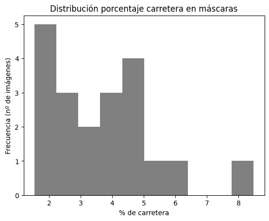
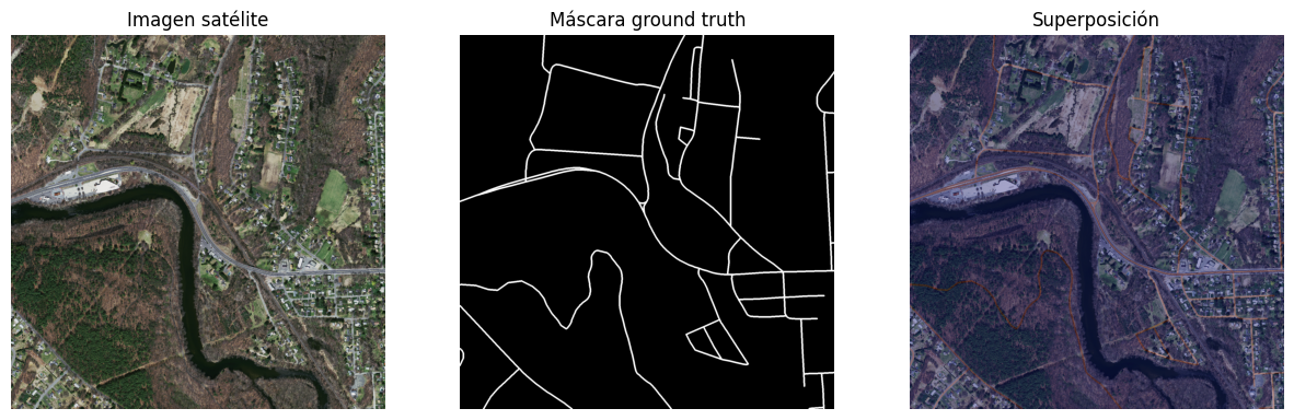
The objective is to produce a binary mask from a 1500×1500 RGB aerial image, where each pixel is classified as “road” or “background”. Ground truth masks feature very thin roads and severe class imbalance (approximately 3–4% road pixels), requiring careful feature representation and evaluation metrics.
- Road average: 3.70%
- Standard deviation: 1.74%
- Min: 1.54%
- Max: 8.48%
Dataset Exploration and Analysis#
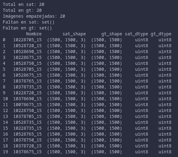
Work is conducted with 20 pairs of satellite image + ground truth mask, previously matched and verified. All images share resolution and data types, with road pixels averaging around 3–4% per image and moderate variability between scenes.
Various contexts are analyzed from representative examples, particularly semi-urban areas with shadows and dense vegetation, to identify conditions where road contrast becomes particularly low.

Classical Feature Engineering#
Color Space Analysis#
The first stage addresses the question of which color channels best distinguish roads. Images are transformed from RGB to HSV, LAB, YCrCb, and HLS spaces, systematically visualizing all channels and comparing road/background contrast.
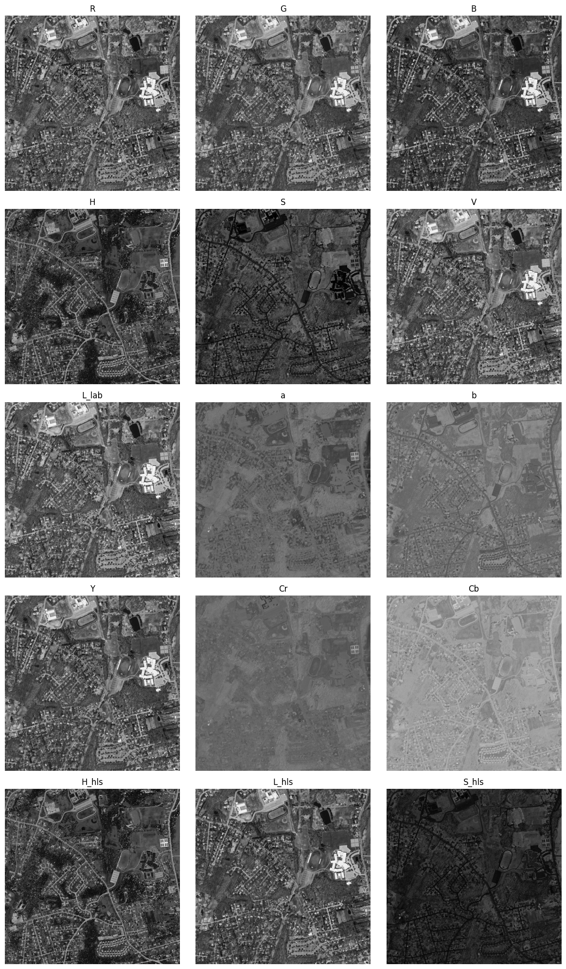
Key findings include:
- H and S (HSV) and H_hls and S_hls (HLS) channels are most effective for road discrimination. b* and Cb provide secondary utility. Other channels contribute little relevant information.
- Channels like a* or Cr render roads nearly invisible and are discarded.
Histogram-Based Thresholding#
On the most promising channels, histogram-dependent thresholds are explored, generating for each channel:
- Intensity histogram.
- Set of thresholds within relevant percentile ranges.
- Resulting binary masks for each threshold value.
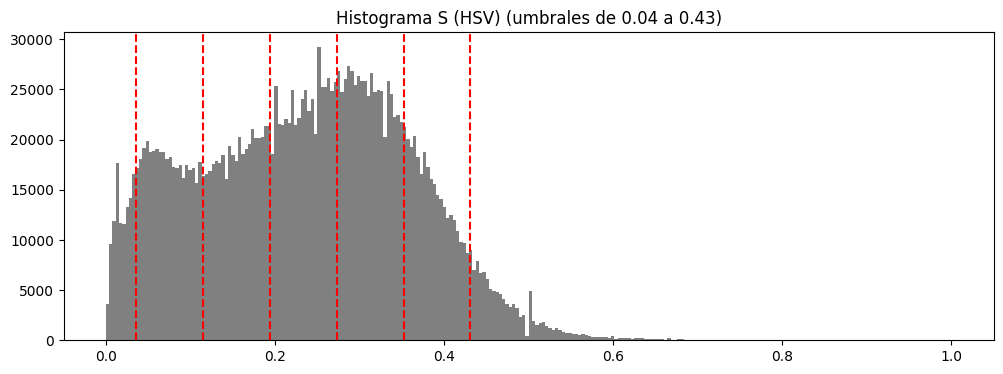
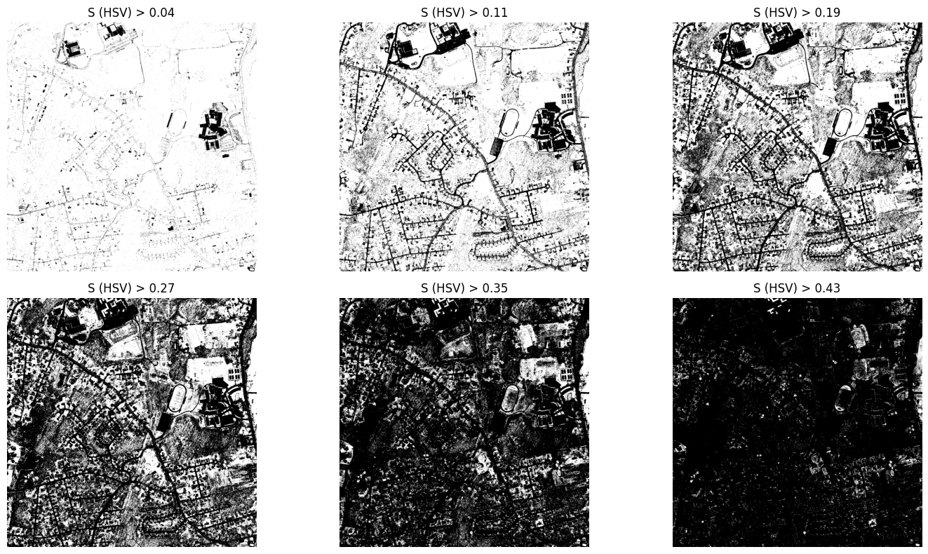
This analysis establishes concrete thresholds, such as:
- S (HSV) ≈ 0.11
- S_hls (HLS) ≈ 0.08
- b* (LAB) ≈ 0.51
- Cb (YCrCb) ≈ 0.50
as suitable starting points for binary mask construction.
Morphological Operations and Cleanup#
Initial binary masks are refined using morphological operators (closing, opening) and small object/hole removal functions to:
- Connect fragmented road segments.
- Eliminate isolated noise and spurious small regions.
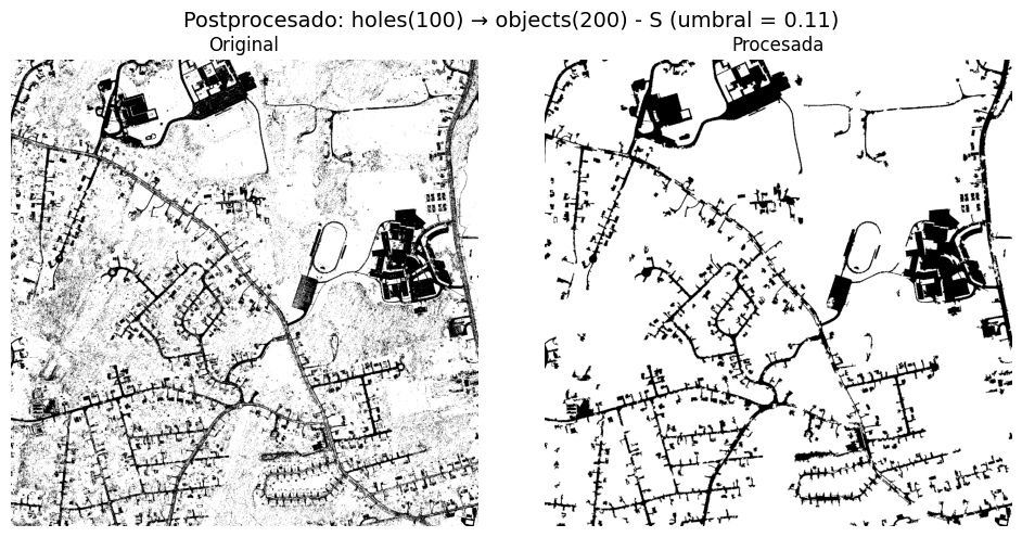
The result is masks where the road network appears more continuous and with reduced noise, for both channels where roads appear dark and where they appear light.
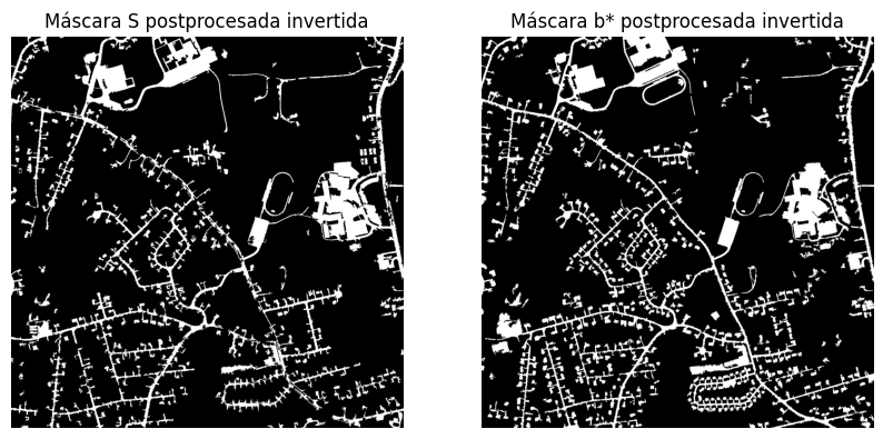
Logical Mask Fusion#
Logical combinations (AND, OR, majority voting) are tested between the best masks (S, S_hls, b*, Cb), both raw and postprocessed versions, seeking to reinforce consistent information across channels and reduce channel-specific noise.
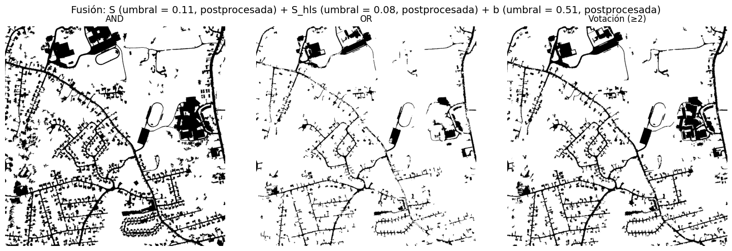
In particular, AND fusion of dark postprocessed masks (S, S_hls, b*) produces a very clean road network, though quantitative improvement over the best individual mask is limited.
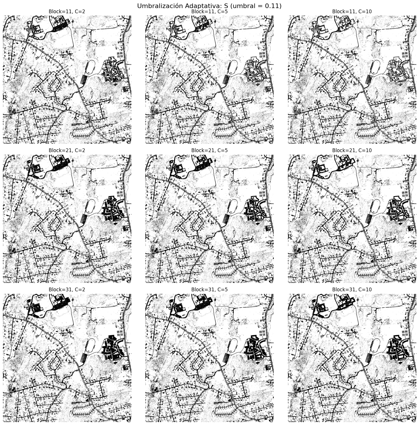
Gradients, Edges, and Adaptive Thresholding#
Edge operators (Sobel, Laplacian, Canny) are evaluated directly on masks, along with adaptive thresholding using different block sizes and C values.
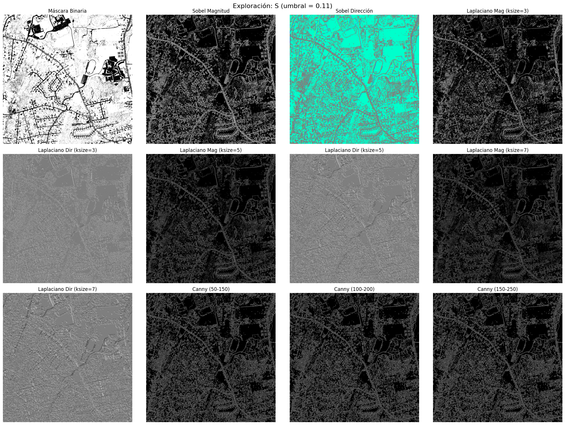
Main observations include:
- Sobel and Laplacian provide complementary information to binary masks on specific channels, capturing finer structures; particularly useful are Sobel magnitude and Laplacian direction (ksize = 5) on postprocessed S and b*.
- Canny identifies the road network but introduces excessive noise for fine segmentation objectives.
- Adaptive thresholding proves especially effective on light-tone channels (H, H_hls, Cb), significantly reducing noise and generating well-defined connected road components; on dark-tone channels, improvements are more limited and channel-dependent.
Best Classical Result Without Deep Learning#
Combining:
- Selected chromatic channels (S, b*, Cb),
- Carefully tuned fixed thresholding,
- Morphological postprocessing,
yields visually reasonable segmentation but remains significantly distant from ground truth when measured with strict metrics like Dice or IoU.
U-Net Segmentation Pipeline#
Feature Volume Construction#
Rather than using only the RGB image, a 17-channel feature volume is constructed per image, where each channel represents a specific feature:
- Normalized RGB channels (R, G, B).
- Binary and postprocessed masks from S, b*, and Cb.
- Derivatives (Sobel magnitude, Laplacian direction).
- Adaptive thresholding versions.
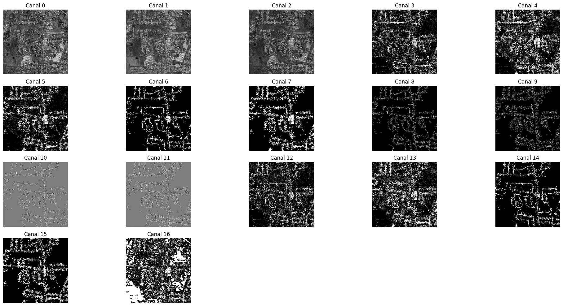
All features are rescaled and resized to 256×256 to enable feasible training on general-purpose GPU/CPU.
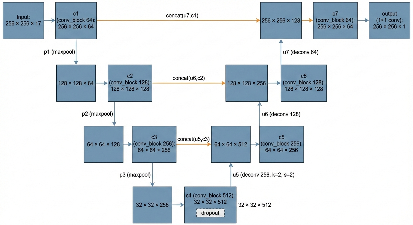
U-Net Architecture#
The segmentation model is based on a U-Net featuring:
- Encoder with convolutional blocks at 64, 128, and 256 filters.
- Bottleneck with 512 filters and
Dropout. - Symmetric decoder with
Conv2DTransposelayers and skip connections from encoder. - Output layer
Conv2D(1, 1)with sigmoid activation producing per-pixel probability.
Loss Function and Metrics#
Given severe foreground-background imbalance, the loss function combines:
Binary Crossentropy (BCE), controlling per-pixel error:
$$ \mathcal{L}{\text{BCE}}(y, \hat{y}) = - \frac{1}{N} \sum{i=1}^{N} \left[ y_i \log(\hat{y}_i) + (1 - y_i)\log(1 - \hat{y}_i) \right] $$
Dice Loss, penalizing prediction-ground truth overlap deficiency:
$$ \mathcal{L}{\text{Dice}}(y, \hat{y}) = 1 - \frac{2 \sum{i=1}^{N} y_i \hat{y}i + \varepsilon}{\sum{i=1}^{N} y_i + \sum_{i=1}^{N} \hat{y}_i + \varepsilon} $$
Total loss function:
$$ \mathcal{L} = \mathcal{L}{\text{BCE}} + \mathcal{L}{\text{Dice}} $$
Evaluation metrics employed are:
Dice coefficient:
$$ \text{Dice}(y, \hat{y}) = \frac{2 \sum_{i=1}^{N} y_i \hat{y}i}{\sum{i=1}^{N} y_i + \sum_{i=1}^{N} \hat{y}_i} $$
IoU (Jaccard index):
$$ \text{IoU}(y, \hat{y}) = \frac{\sum_{i=1}^{N} y_i \hat{y}i}{\sum{i=1}^{N} y_i + \sum_{i=1}^{N} \hat{y}i - \sum{i=1}^{N} y_i \hat{y}_i} $$
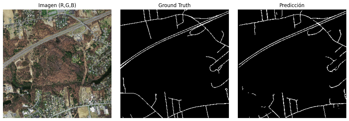
Training, Validation, and Results#
The dataset is split into training and validation subsets. To improve generalization, data augmentation applies geometric and photometric transformations (rotations, flips, brightness/contrast changes, blur, noise, elastic deformations).
Early stopping monitors validation loss to prevent overfitting and select the best model.
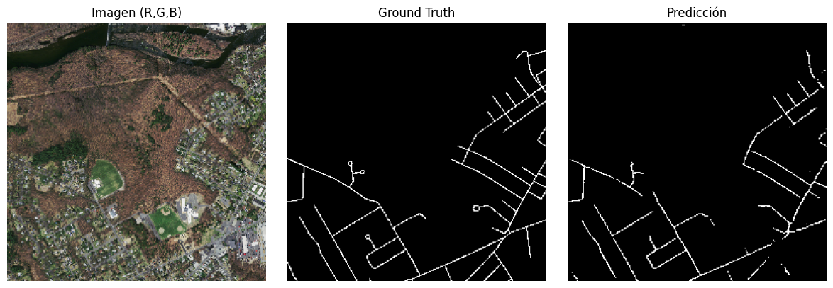
Quantitative results across the 20 images are approximately:
- U-Net Dice average: ≈ 0.69
- U-Net IoU average: ≈ 0.53
- Best classical Dice average: ≈ 0.34
- Best classical IoU average: ≈ 0.21
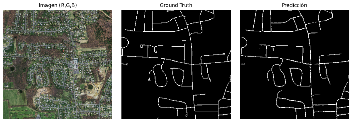
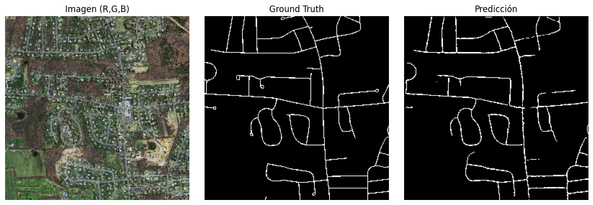
Visually, U-Net produces more continuous masks with better road network alignment and greater ability to fill weak or partially occluded road segments.
Conclusions and Contributions#
- The classical feature engineering pipeline (color spaces, thresholding, morphology, mask fusion) provides interpretable segmentations and serves as solid foundation for problem understanding.
- However, when quantitative ground truth approximation is required, the U-Net trained on enriched feature volumes offers clear improvement in both Dice and IoU.
- The approach emphasizes explainability: each input volume channel corresponds to a visually interpretable transformation, facilitating error analysis and technical discussion with both engineering and management profiles.
Technology Stack and Organization#
- Language and libraries: Python 3.12, NumPy, SciPy, scikit-image, OpenCV, TensorFlow/Keras, Albumentations, Matplotlib.